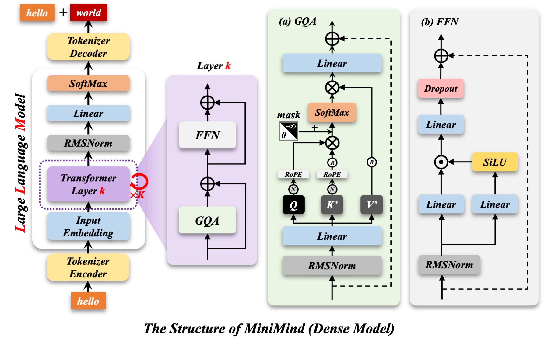
MiniMind publishes a small language model’s architecture and training process. The current MiniMind-3 Dense model has about 64 million parameters. A separate MoE version has around 198 million total parameters and 64 million active parameters. A useful first pass is to run the released model, then reproduce pretraining and supervised fine-tuning, or SFT, with the smaller datasets.
Check the environment and model generation
Use a separate Python environment, clone the repository and install its dependencies. The README lists Python 3.10.16, Ubuntu 20.04 and CUDA 12.2 as a reference setup, not a universal minimum. PyTorch installation is commented out in the dependency file, so choose a PyTorch build compatible with your hardware and CUDA environment separately.
git clone --depth 1 https://github.com/jingyaogong/minimind
cd minimind
pip install -r requirements.txt
For NVIDIA GPU training, confirm that torch.cuda.is_available() returns True before downloading training data. Speed and compatibility differ on CPU and other backends; the RTX 3090 timing does not transfer to them. Record the repository revision so commands and settings can be traced later.
Start a conversation with released weights
Download the Transformers-format MiniMind-3 model into the repository root. One documented route uses ModelScope, followed by the evaluation script:
modelscope download --model gongjy/minimind-3 --local_dir ./minimind-3
python eval_llm.py --load_from ./minimind-3
This uses existing weights to check dependencies, tokenizer loading and generation. Native PyTorch weights produced by training are saved under out and loaded differently. A Transformers model directory and an individual .pth file are not interchangeable.
Prepare two datasets and train in sequence
For a first reproduction, place pretrain_t2t_mini.jsonl and sft_t2t_mini.jsonl in the repository’s dataset directory. Pretraining uses text examples; SFT uses conversations. Having the same file extension does not make their sample fields interchangeable.
Enter trainer, run pretraining and then run SFT. These commands use the scripts’ current defaults, including two epochs for each stage:
cd trainer
python train_pretrain.py
python train_full_sft.py
SFT defaults to loading the pretrain weights. The default hidden size is 768, and model settings must match between stages. Default outputs include out/pretrain_768.pth and out/full_sft_768.pth, relative to the repository root.
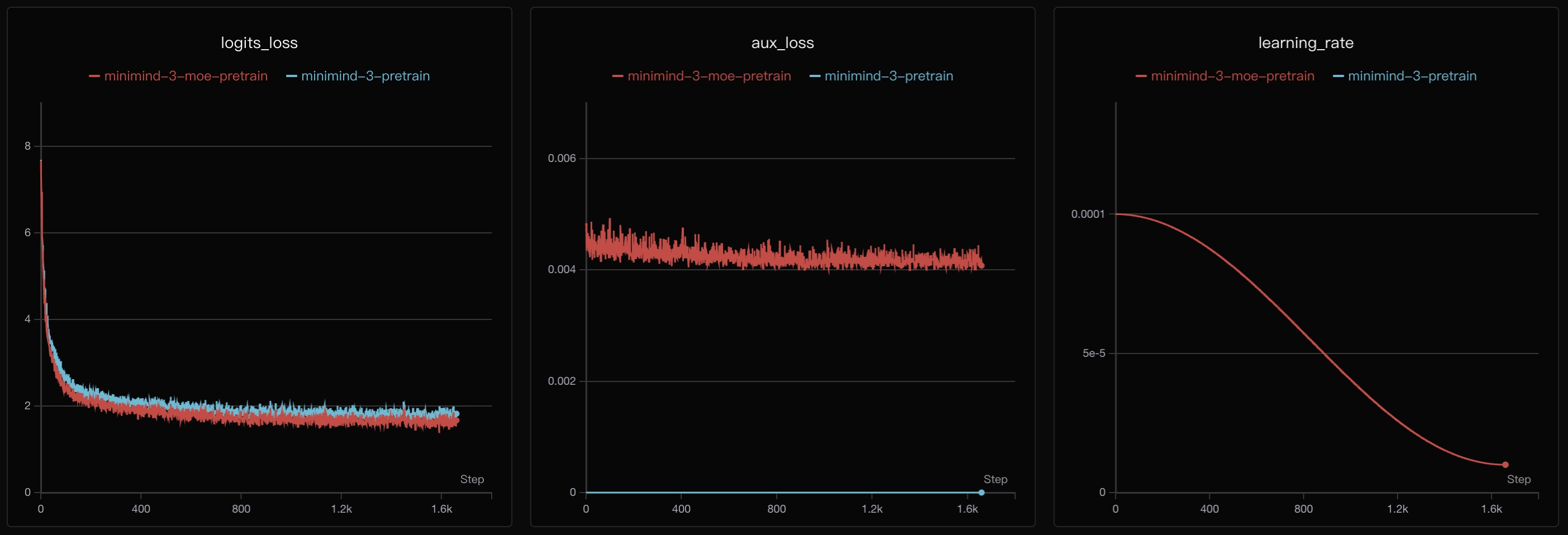
This chart comes from the project’s Dense and MoE pretraining experiments. Check how loss and learning rate change, then inspect your own log for timing and failures. Separate held-out examples are needed to see whether a trained model can answer your target questions.
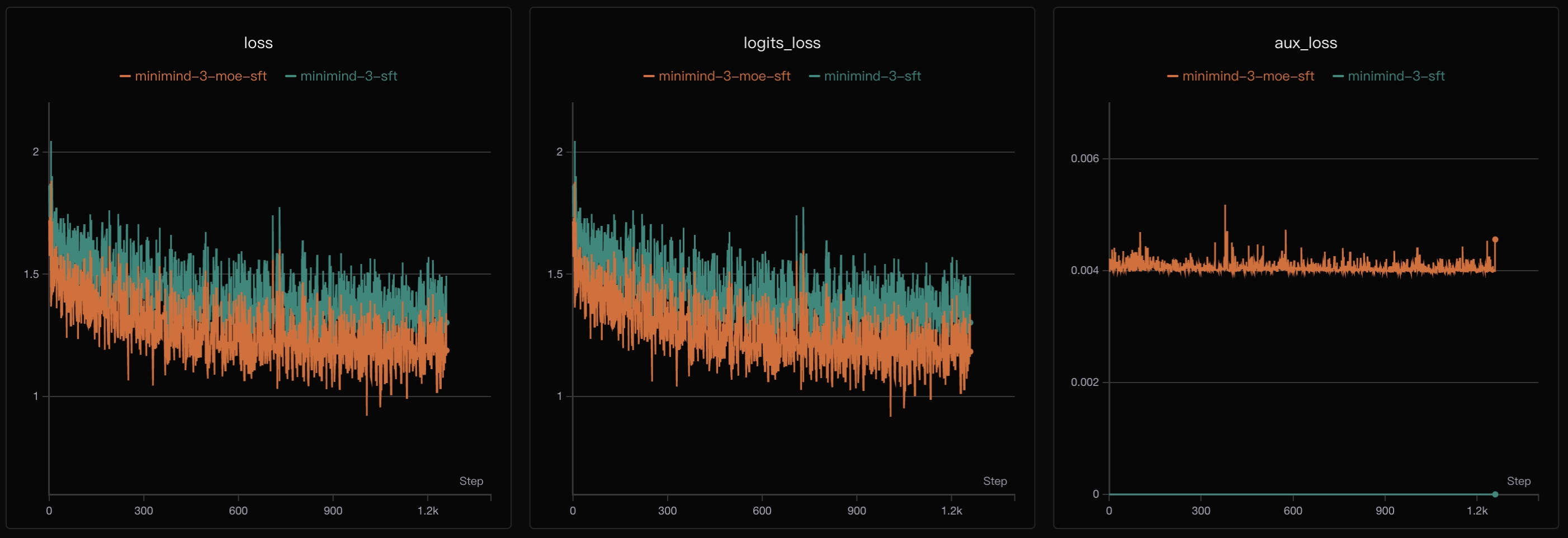
The SFT chart also comes from the repository. Pretraining and SFT optimize different data objectives, so the numerical height of these two plots is not a direct comparison of answer quality. Training visualization options can be enabled to record your own runs.
Keep progress and inspect your trained model
The scripts save inference weights and training-resume checkpoints. Add --from_resume 1 to the original training command to recover existing progress after interruption. Resume files under checkpoints include training state and serve a different purpose from inference weights.
After SFT finishes, return to the repository root and load your model:
cd ..
python eval_llm.py --load_from ./model --weight full_sft
Keep a fixed set of prompts: unfamiliar wording, questions the model should decline and simple factual questions. Recording mistakes and generation speed makes data or training problems easier to spot than selecting one fluent conversation.
A chat interface and further experiments
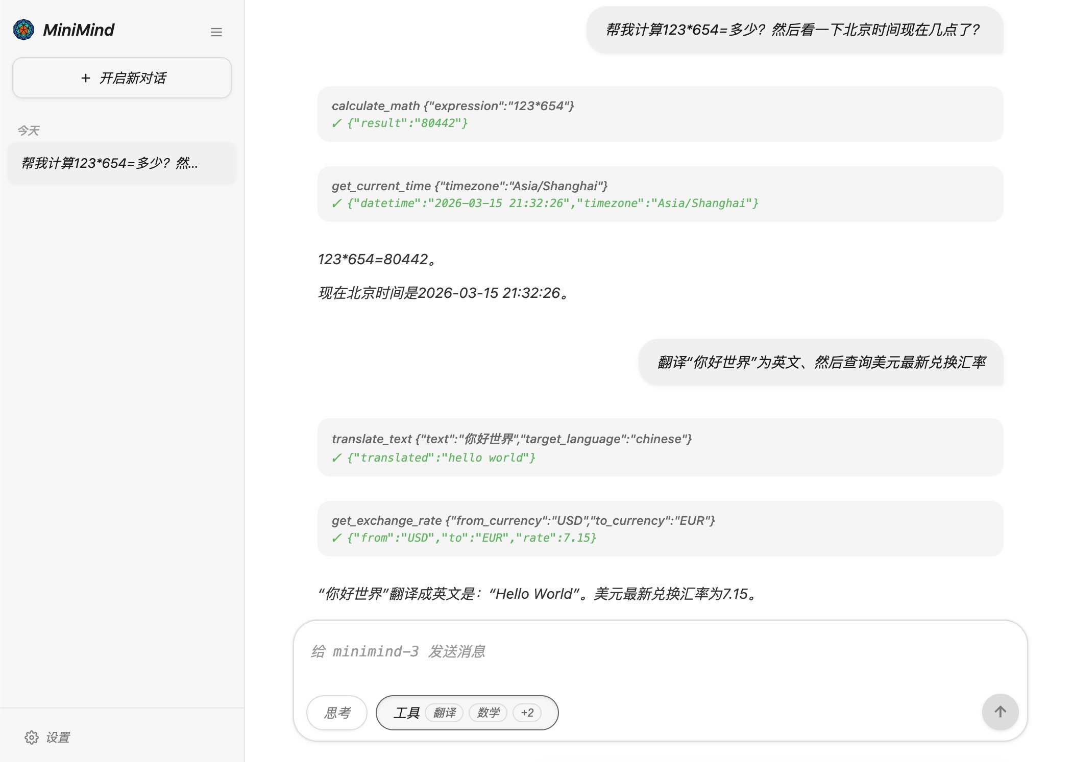
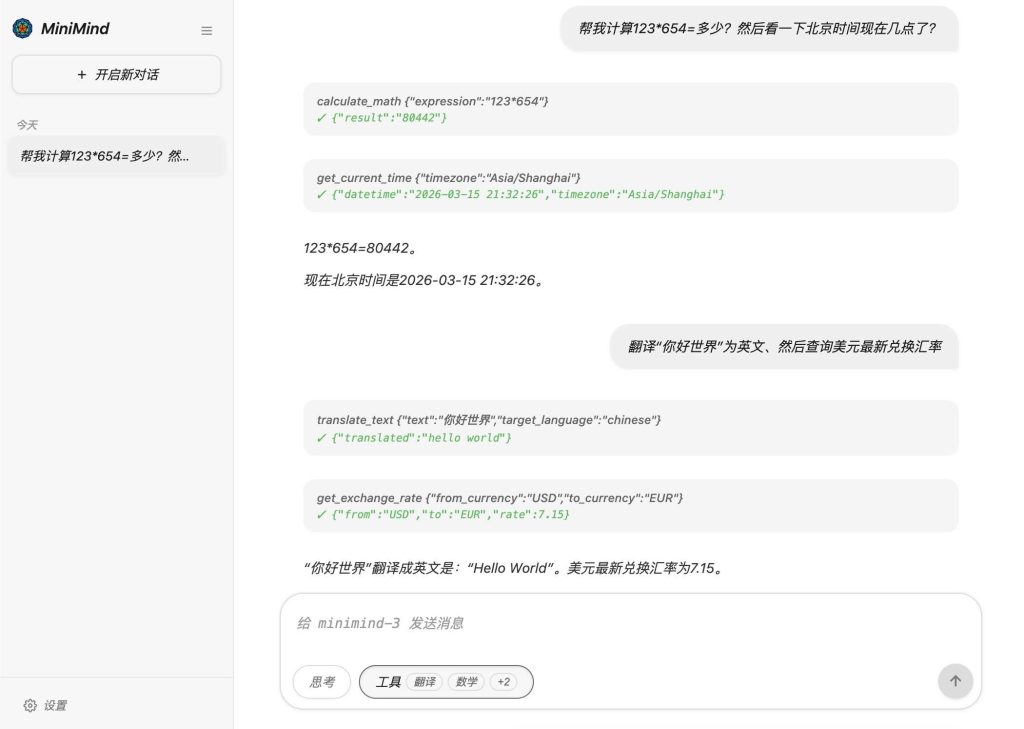
The repository provides a Streamlit WebUI. With Transformers-format weights, copy the model directory into scripts so the interface can discover it, then run streamlit run web_demo.py from that directory. The screenshot is the author’s tool-call example; it does not establish the accuracy of the tools or model on real tasks.
After completing the basic path, explore LoRA, DPO, GRPO or Agentic RL individually. Each introduces different data and objectives. Adding one stage at a time helps identify which change affected the answers.
The project’s two-hour, three-yuan example covers one SFT epoch on a single RTX 3090 and its corresponding GPU rental. It is not a fixed budget for the entire reproduction. This guide checks the code and public documentation; no training run was performed for the article. All illustrations are original project images.
Resources: GitHub project · Dependencies · Pretraining script · SFT script · Inference script · WebUI · Apache 2.0 license
Copy the link to save or share this article.